Inference with Neural Networks

In this project, you will use generative backpropagation to infer the state of a dynamical system from image-based observations, and you will train a model of the dynamical system.

Instructions:

Learn how to train a generative neural network with unsupervised learning using a collection of images. (A generative neural network is one that generates images, rather than consumes them.) Let V refer to a latent matrix of inputs. Let W refer to the weights of your network. You will initialize V to contain all zeros. You will initialize W with small random values. Then, you will use gradient descent to refine both V and W until the neural network can generate images like X. To begin, you will need to choose the number of dimensions to use in V. I will call this variable k.

Here is some pseudo-code to train an MLP in this manner:
```
void train_unsupervised(const Matrix& X)
{
    n = X.rows();
    Let V be an n-by-k matrix.
    Set all the values in V to 0.0;
    double learning_rate = 0.0001;
    for(size_t j = 0; j < 100; j++)
    {
        for(size_t i = 0; i < 1000000; i++)
        {
            t = rand.next(X.rows());
            features = V[t]
            label = X[t]
            predict(features, pred);
            compute the error on the output units
            do backpropagation to compute the errors of the hidden units
            compute the blame terms for V[t]
            use gradient descent to refine the weights and bias values
            use gradient descent to update V[t]
        }
        print(to_str(j + 1) + "%\n");
    }
}
```
Note that this is very similar to the supervised way we train an MLP. The main difference, which I have hilighted in red, is that the inputs, V, are now latent, so we update them with gradient descent too. Here is how we calculate the gradient with respect to the inputs:

Let $\mathbf{v}_i$ be an element of the input vector.
Let $E$ be the squared error.
Let $e_j$ be the blame term on unit $j$.
Let $w_{i,j}$ be the weight between them.
Then the gradient of the error with respect to $\mathbf{v}_i$ is $\nabla_{\mathbf{v}_i}E=-\sum_j w_{i,j}e_j$.

In other words, the blame term for the inputs is just the blame terms for the net of the input layer multiplied by the weights of the input layer.

In this project, we will train your unsupervised MLP using a collection of images. Our generative model will learn these images as continuous functions, rather than as collections of pixels. (I will refer to the width and height of the images as "width" and "height".) Here is a training method to do this. (Differences from the pseudo-code above are highlighted in red.)

void train_with_images(const Matrix& X)
{
    channels = X.cols() / (width * height);
    Initialize the MLP to have channels output units (not X.cols() outputs).
    n = X.rows();
    k = number of degrees of freedom in the system;
    Allocate an n-by-k matrix, V, to hold intrinsic vectors
    V.setAll(0.0);
    double learning_rate = 0.1;
    for(size_t j = 0; j < 10; j++)
    {
        for(size_t i = 0; i < 10000000; i++)
        {
            t = rand.next(X.rows());
            p = rand.next(width);
            q = rand.next(height);
            features = a vector containing p/width, q/height, and V[t]
            s = channels * (width * q + p);
            label = the vector from X[t][s] to X[t][s + (channels - 1)]
            pred = predict(features);
            compute the error on the output units
            do backpropagation to compute the errors of the hidden units
            compute the blame terms for V[t]
            use gradient descent to refine the weights and bias values
            use gradient descent to update V[t]
        }
        learning_rate *= 0.75;
    }
}

Take some time to understand the red parts.

I built a model of a simple crane system that moves with two degrees of freedom. (In other words, k=2):

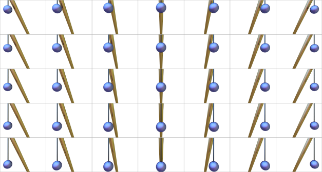
This crane is equipped with 4 possible actions: a=left, b=right, c=up, d=down. I initialized the crane to the center position. I then performed 1000 random actions to this crane. I stored the actions in a file named "actions.arff". Before performing each action, I used a ray-tracer to take a virtual picture of my crane. Each picture contained 64x48 pixels, and each pixel contained 3 channel values ranging from 0-255. I converted each picture to a 9216-dimensional vector (64*48*3=9216) and stored it in a file named "observations.arff". I stored the actions in a file named "actions.arff". Download this zip archive, containing these two datasets.

For example, here are the first 16 images in observations.arff with the first 15 actions in actions.arff between them:

a (left)

a (left)

b (right)

a (left)

a (left)

d (down)

a (left)

a (left)

a (left)

c (up)

b (right)

a (left)

c (up)

a (left)

b (right)

Make a 3-layer MLP with a 4-12-12-3 topology. (Two inputs for the pixel-coordinates, and two inputs for the state of the crane. Three outputs for the three channel values: red, green, and blue.) Load observations.arff into a matrix, X, and pass it to your train_with_images method to reduce it to a 2-dimensional matrix of intrinsic values, V. Doing this will also train your MLP to map from V->X. This is called the observation function. (This step takes about 10 minutes on my laptop's throttled 2.2Ghz i7 processor. I recommend printing some indication of progress while it trains.) Note that the pixel values range from 0-255. Since an MLP that uses the tanh activation function in the output layer can only predict output values from 0-1, you need to do some normalization. It might be easiest to just divide all observation values by 256 after you load them, so you don't have to worry about normalizing them. (Just don't forget to multiply your predictions by 256 again before you try to generate an image, or it will come out solid-black.)
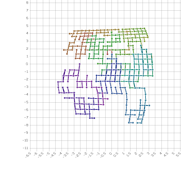
Here is a plot of V that I obtained with my unsupervised MLP. I connected each point with the next point, so you could see how the crane wanders through its state space. I plotted beginning with red, then passing through yellow, green, cyan, and ending with blue:

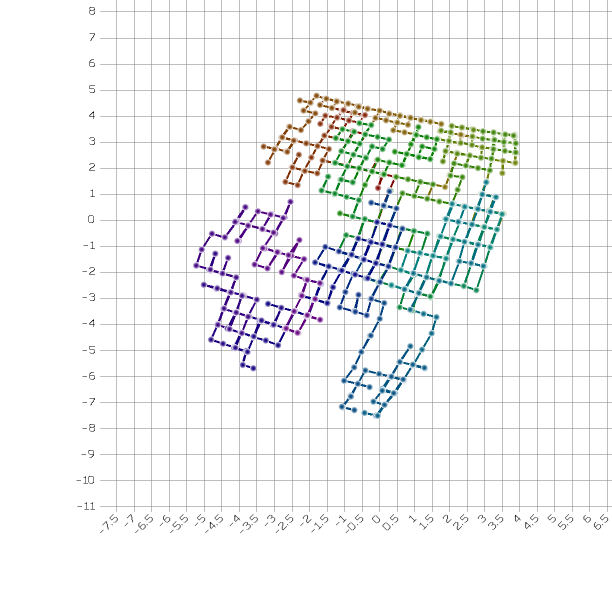
Your results may be rotated, skewed, or different in some other way from my results, because the MLP is free to represent the intrinsic values in any way that it finds convenient, as long as it can find a mapping to the observations. You should, however, see a similar structure. Here is a plot of the state that I get when I run it again with a different random seed:

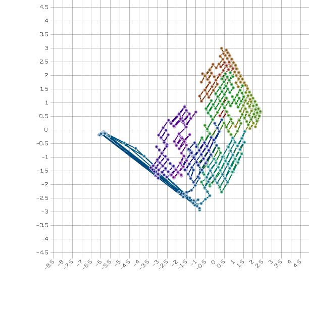
Here is a plot of the actual ground-truth states that were withheld from the model during training:

Sometimes, you might get a small number of points that are obviously misplaced. This means it fell into a local optimum. I will not be concerned about this. If you rerun it with a different random seed, it will probably not happen again.

Plot your intrinsic values, V. Draw a line between each point and the next point. Save your plot as "intrinsic.svg" or "intrinsic.png".

Make another MLP with just one hidden layer containing 6 units. Train this one as a supervised MLP to predict how actions change the state. This is called the transition function. A good way to train the transition function is to generate some new data from V. This new data will have one fewer rows than V. The features of this data consist of each of the rows in V (except the last one), and the action that was performed in that state.

The labels consist of the next row in V, because you are trying to predict the state that will follow. (I found that I obtain better results when I predict the difference between the next state and the current state, and then add this difference to the current state to predict the next one.) Remember, your MLP can only predict values between 0 and 1, so you will need to do some normalization to get the values within a suitable range.) Train your MLP on this new data, so it can predict how the state changes each time you perform an action.

Initialize the state vector to the first row in V. (This is the state where the crane is in the central position.) Feed this state through the observation function to generate a predicted image and save it as "frame0.svg" or "frame0.png". This image should depict the crane in its central starting position. Use your model to predict how v changes as you perform action 'a' five times. After each action, save the predicted images as "frame1.svg", "frame2.svg", etc. Next, perform action 'c' five times. After each action, save the images as "frame6.svg", "frame7.svg", etc. (In other words, simulate moving the crane left five times, and then up five times.)

Here is some pseudocode to generate an image. (This pseudocode assumes that p and q come first in the inputs to your observation function, and the state comes next. If you did it differently, some adjustments may be necessary to make this consistent with your implementation.)
```
unsigned int rgbToUint(int r, int g, int b)
{
	return 0xff000000 | ((r & 0xff) << 16)) |
		((g & 0xff) << 8) | ((b & 0xff);
}

void makeImage(Vec& state, const char* filename)
{
	Vec& in;
	in.resize(4);
	in[2] = state[0];
	in[3] = state[1];
	Vec& out;
	out.resize(3);
	Image im;
	im.resize(w, h);
	for(size_t y = 0; y < h; y++)
	{
		in[1] = (double)y / h;
		for(size_t x = 0; x < w; x++)
		{
		  in[0] = (double)x / w;
		  predict(in, out);
		  unsigned int color = 
		    rgbToUint(out[0] * 256, out[1] * 256, out[2] * 256);
		  im.setPixel(x, y, color);
		}
	}
	im.savePng(filename);
}
```
Here are the results that I get:
Frame 0:

Frame 5:

Frame 9:

Hints:

I strongly recommend using Java or C++ for this assignment. Python is just too slow with floating point operations. No, numpy will not make it fast. In Java or C++ it only takes about 10 minutes to run. In Python, it takes hours.

When you use division, be careful not to use integer arithmetic when you should be using floating-point arithmetic. In integer arithmetic, 51/64=0.

If your crane moves in the wrong direction, there is something wrong with your transition function. Did you use a one-hot representation for the nominal action? A continuous representation would not work well. If it moves in the right direction, but then stops when it should keep going, you probably didn't normalize the intrinsic values to fall within a range your transition function could handle. You might want to wrap your transition function in a filter with Normalize and NomCat to handle these issues.

Java examples for working with images:

import java.awt.image.BufferedImage;
import java.io.File;
import javax.imageio.ImageIO;
import java.io.IOException;

// Load a image from a file
BufferedImage image = ImageIO.read(new File(inputFilePath));

// Make a new image
BufferedImage newimage = new BufferedImage(width,
	height, BufferedImage.TYPE_INT_ARGB);

// Read a pixel
Color c = new Color(image.getRGB(x, y));
int greenChannel = c.getGreen();

// Set a pixel (0xAARRGGBB)
image.setRGB(x, y, 0xff00ff00);

// Write the image to a PNG file
ImageIO.write(image, "png", new File(outputFilePath));

Here is a simple C++ program that writes a PNG image.

To help you debug step 3, here is some debug spew from my implementation. In order to enable deterministic results, I made the following adjustments:
- I initialized the weights in each layer with the values 0.007*r+0.003*c, where r and c are the row and column indexes.
- I initialized each element in the bias with 0.001*i, where i is the element index.
- I changed these lines:
```
t = rand.next(X.rows());
p = rand.next(width);
q = rand.next(height);
```
  to
```
t = i % 1000;
p = (i * 31) % 64;
q = (i * 19) % 48;
```
- I changed
```
for(int i = 0; i < 10000000; i++)
```
  to
```
for(int i = 0; i < 100; i++)
```
Unfortunately, these changes are sufficient to ruin the results. However, if you test that your numbers match mine, then undo these changes, you should expect it to work.

The nomcat and normalizer transforms depend on the meta-data to determine which attributes to transform. If you use these with your transition model, make sure that the data you use to train it contains valid meta-data. If you manually copy values from the original matrices, the meta-data may be lost. The copyBlock method, however, is designed to preserve the meta-data.