Back to the table of contents

Previous Next

Examples of dimensionality reduction

This document shows examples of using dimensionality reduction techniques.

Attribute selection

Attribute selection is one of the simplest dimensionality reduction techniques. It involves deciding which attributes (or columns) are the least salient, and throwing them out. In this example, we'll use the hepatitis dataset (which can be obtained at MLData.org). Here is a simple command that will generate an ordered list of attributes:

	waffles_dimred attributeselector hepatitis.arff

The output of this command is:

	Attribute rankings from most salient to least salient. (Attributes are zero-indexed.)
	16 ALBUMIN
	13 BILIRUBIN
	17 PROTIME
	1 SEX
	6 ANOREXIA
	15 SGOT
	5 MALAISE
	9 SPLEEN_PALPABLE
	3 ANTIVIRALS
	11 ASCITES
	4 FATIGUE
	8 LIVER_FIRM
	18 HISTOLOGY
	12 VARICES
	14 ALK_PHOSPHATE
	0 AGE
	7 LIVER_BIG
	2 STEROID
	10 SPIDERS

This tool works by normalizing all the values, and then training a logistic regression model to predict the label. The attribute that is assigned the smallest weight, which in this case was column 10 (SPIDERS), is dropped from the data, and the process is repeated. (I presume this is a reference to the feeling that spiders are crawling on one's skin. Since the mere mention of that concept causes many people to begin scratching, it makes sense that this attribute would be a poor predictor of serious liver problems, whereas some of the more measurable conditions tend to be the best predictors.)

Now, let's generate a dataset containing only the three most salient features.

	waffles_dimred attributeselector hepatitis.arff -out 3 hep.arff

Let's verify that the new dataset now only contains three feature attributes.

	waffles_plot stats hep.arff

The output of this command is:

	Filename: hep.arff
	Patterns: 155
	Attributes: 4 (Continuous:3, Nominal:1)
	  0) ALBUMIN, Type: Continuous, Mean:3.8172662, Dev:0.65152308, Median:4, Min:2.1, Max:6.4, Missing:16
	  1) BILIRUBIN, Type: Continuous, Mean:1.4275168, Dev:1.212149, Median:1, Min:0.3, Max:8, Missing:6
	  2) PROTIME, Type: Continuous, Mean:61.852273, Dev:22.875244, Median:61, Min:0, Max:100, Missing:67
	  3) Class, Type: Nominal, Values:2, Most Common:LIVE (79.354839%), Entropy: 0.73464515, Missing:0
	     20.645161% DIE
	     79.354839% LIVE

Yep, it only has 3 features. Okay, let's see how well we can predict whether the person will live or die using just these three features, and we'll compare it with the original dataset. We'll also specify a seed for the random number generator, so our results can be reproduced.

	waffles_learn crossvalidate -seed 0 hepatitis.arff bag 50 decisiontree end
	waffles_learn crossvalidate -seed 0 hep.arff bag 50 decisiontree end

With the original dataset, we get 79.1 percent accuracy. With the smaller dataset, we get 79.5 percent accuracy. Not too shabby! (Often, the accuracy goes down just a little bit, and we claim success just because we can achieve similar accuracy using fewer features, and therefore less computation.)

Principal component analysis

In this example, we will use PCA to reduce the dimensionality of the same dataset. We only want to reduce the dimensionality of the features, so we will begin by stripping off the labels. First, we do:

	waffles_plot stats hepatitis.arff

This command shows us that column 19 is the label column. So, let's drop that column:

	waffles_transform dropcolumns hepatitis.arff 19 > hep_features.arff

Now, since PCA expects only continuous features, we need to convert all of the nominal attributes to continuous values. This is done by representing each nominal value using a categorical distribution:

	waffles_transform nominaltocat hep_features.arff > hf_real.arff

Now, let's use PCA to reduce the dimensionality of the data. Let's use 3 dimensions, since that worked out so well in the previous example.

	waffles_dimred pca hf_real.arff 3 > hf_reduced.arff

Then, we'll attach the labels to the reduced features.

	waffles_transform dropcolumns hepatitis.arff 0-18 > hep_labels.arff
	waffles_transform mergehoriz hf_reduced.arff hep_labels.arff > hep_final.arff

If we examine the data, we will see that it indeed contains three features and one label.

	waffles_plot stats hep_final.arff

This command will output the following:

	Filename: hep_final.arff
	Patterns: 155
	Attributes: 4 (Continuous:3, Nominal:1)
	  0) Attr0, Type: Continuous, Mean:1.2698086e-13, Dev:89.14132, Median:-25.735051, Min:-79.748934, Max:556.56446, Missing:0
	  1) Attr1, Type: Continuous, Mean:5.8952126e-14, Dev:45.301948, Median:-7.1158747, Min:-77.957909, Max:191.04956, Missing:0
	  2) Attr2, Type: Continuous, Mean:1.5815306e-15, Dev:16.968467, Median:0.26878276, Min:-43.309528, Max:65.561348, Missing:0
	  3) Class, Type: Nominal, Values:2, Most Common:LIVE (79.354839%), Entropy: 0.73464515, Missing:0
	     20.645161% DIE
	     79.354839% LIVE

So, let's see how well we can predict using this dataset:

	waffles_learn crossvalidate -seed 0 hep_final.arff bag 50 decisiontree end

It gets 75.5 percent accuracy. Apparently attribute selection is a better way to go with this dataset. Often, PCA is a better choice, but the numbers say otherwise in this case.

Non-linear dimensionality reductions (NLDR)

In this section, we will give examples of non-linear dimensionality reduction.

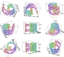
To begin, let's generation 2000 points that lie on the surface of a Swiss roll manifold.

	waffles_generate manifold 2000 "y1(x1,x2) = (8*x1+2) * sin(8*x1); y2(x1,x2) = (8*x1+2) * cos(8*x1); y3(x1,x2) = 12 * x2" > sr.arff

Of course, you could change those formulas to specify any sort of manifold that you want to sample. Since the Swiss roll is such a common manifold for testing NLDR algorithms, we also provide a convenience method, so you don't have to remember those formulas.

	waffles_generate swissroll 2000 -cutoutstar -seed 0 > sr.arff

Note that we specified a random seed, so that our results will be reproduceable. Also, we added a special switch that prevents samples from being taken in a star-shaped region of the manifold. Why? Because it helps with visualizing the quality of the results.

Next, let's visualize our data.

	waffles_generate 3d sr.arff -blast -pointradius 300

The "-blast" flag says to visualize this data from several different random points of view. It is useful when you don't know the best point from which to view your data.

Then, we'll use a few different algorithms to reduce this data into two dimensions.

	waffles_dimred pca sr.arff 2 > pca.arff
	waffles_plot scatter -aspect row pca.arff 0 1 -thickness 0 > pca.svg

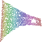
	waffles_dimred isomap sr.arff 14 kdtree 2 > isomap.arff
	waffles_plot scatter -aspect row isomap.arff 0 1 -thickness 0 > isomap.svg

	waffles_dimred lle sr.arff 14 kdtree 2 > lle.arff
	waffles_plot scatter -aspect row lle.arff 0 1 -thickness 0 > lle.svg

	waffles_dimred breadthfirstunfolding sr.arff 14 kdtree 2 -reps 20 > bfu.arff
	waffles_plot scatter -aspect row bfu.arff 0 1 -thickness 0 > bfu.svg

	waffles_dimred manifoldsculpting sr.arff 14 kdtree 2 > ms.arff
	waffles_plot scatter -aspect row ms.arff 0 1 -thickness 0 > ms.svg

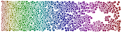
Of our NLDR algorithms, Manifold Sculpting tends to give the best results with most problems, although with many problems it is necessary to use a slower scaling rate than the default in order to get good results. Breadth First Unfolding tends to be the fastest NLDR algorith, often by a large amount, and it usually gives decent results.

Previous Next

Back to the table of contents